![[Artist's Concept of AXAF]](/images/axaf.gif)
|
|
CXO Project Science:
|

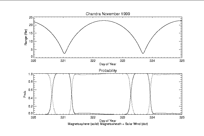
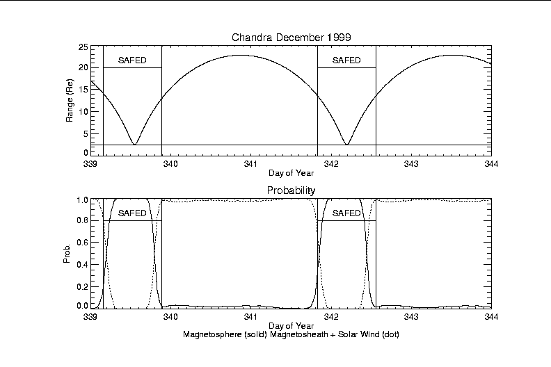
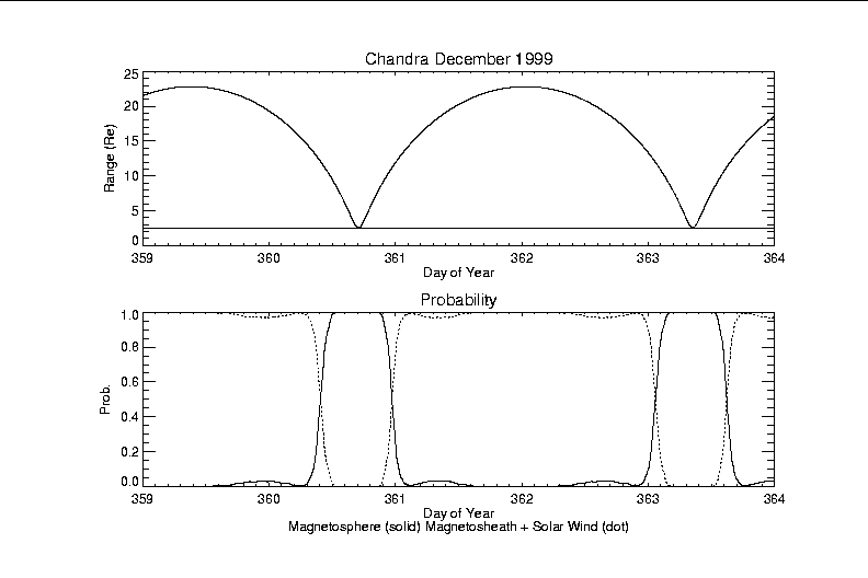
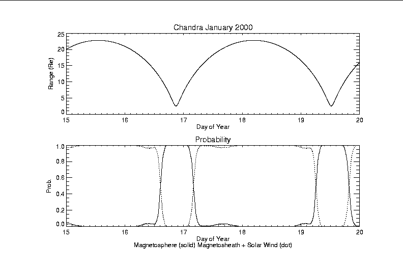
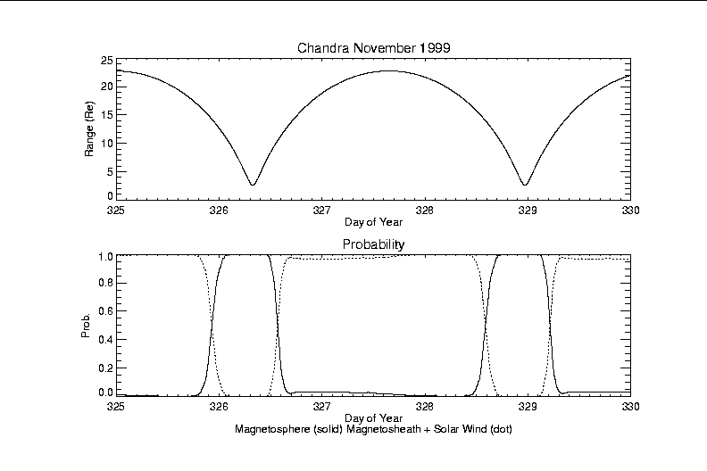
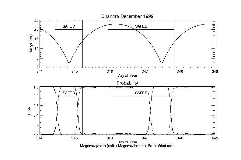
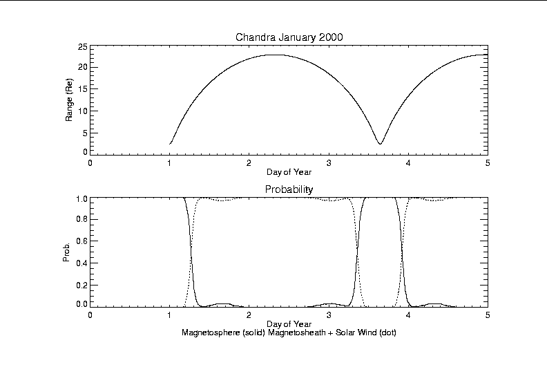
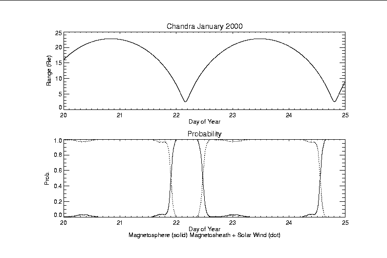
 solar wind,
magnetosheath, or
magnetosphere.
solar wind,
magnetosheath, or
magnetosphere.
The orbits used in the analysis are obtained by propagating NORAD two-line element sets with an SDP4 analytical propagator. Satellite Tool Kit (STK 4.1) software is used to implement the propagation in Geocentric Equatorial Inertial (GEI) coordinates, which are then converted to Geocentric Solar Ecliptic (GSE) coordinates. This gives the satellite position and radial distance in GSE coordinates as a function of time for use in the probability calculations described below. The resulting ephemeris was compared agains the timeline provided by Shanil Virani (CXO/SAO) on 22 December 1999 and found to agree within approximately 500 km altitude and 5-6 minutes in time. Further verification will be required to ensure that the orbit propagation software is compatible with that used by the Chandra program in producing ephemerides for time tagging satellite commands.
The solar-wind model is based upon IMP-8 measurements for 1992 (a period of solar maximum activity). The IMP-8 data does not include the interplanetary magnetic field (IMF) data associated with the plasma parameter data. Instead, typical Parker spiral IMF values were used for the cases examined here. The Bz-component of the field is set to 0, which provides conservative predictions of the bow shock and magnetopause stand-off distances from Earth.
The bow-shock model used is adapted from Bennett et al. ``A Model for the Earth's Distant Bow Shock;'' the magnetopause-boundary model is based upon Petrinic & Russell ``Factors Controlling the Shape and Size of the Post-Terminator Magnetopause.'' The location and shape of the Earth's bow shock and magnetopause are controlled by the solar-wind dynamic pressure and the orientation of the IMF. Both models use solar-wind plasma parameters (number density and flow velocity) and magnetic-field orientation as input.
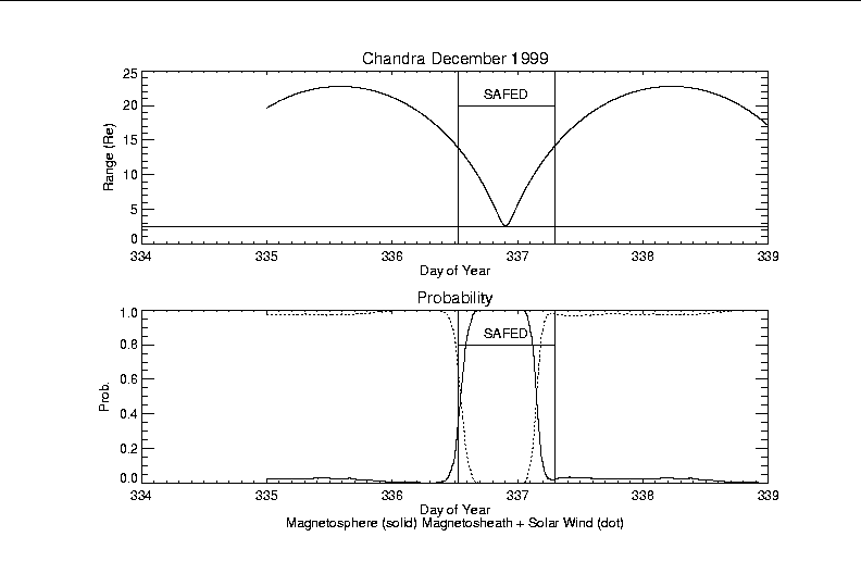
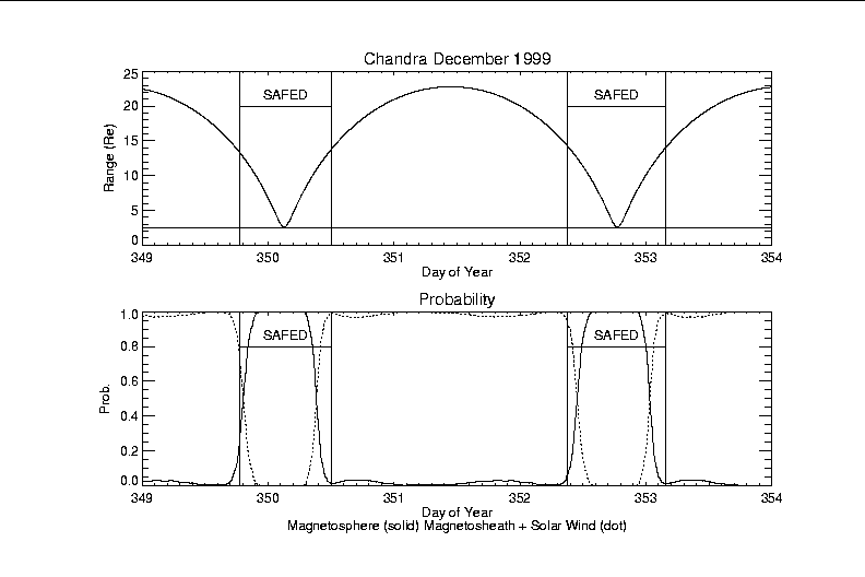
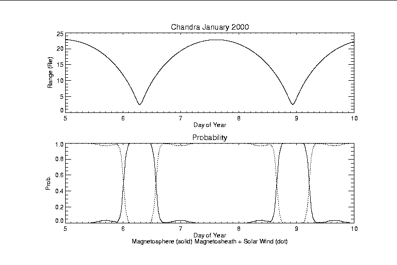
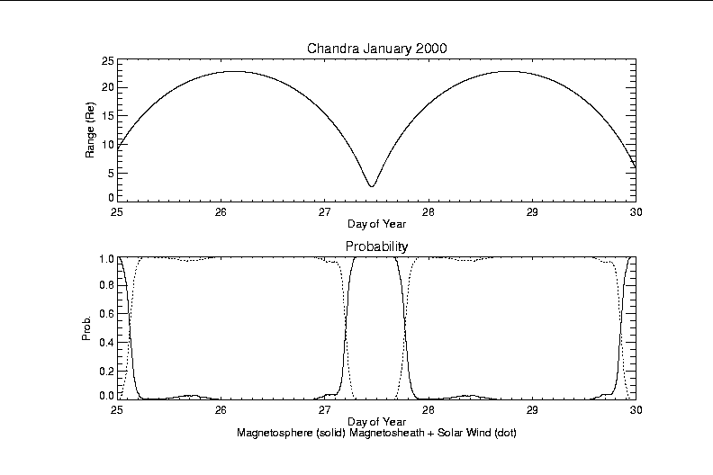
The simulation proceeds as follows: A uniform random draw is made on the fractional day of year for selection of the solar-wind plasma parameters. These solar wind conditions are then used to determine the phenomenological region (solar wind, magnetosheath, magnetosphere) at which each point in the ephemeris is located. Counters track the number of times each satellite location encounters a given region. This process is repeated for the specified number of random draws, in this case, 1000. The probability that a given location in space is in one of the three regions is then simply the fraction of encounters with that region. In the future, it may be desirable to increase the number of random samples to sample more fully the parameter space of variations in the solar-wind plasma parameters.
Currently (2000 January), Chandra's orbit crosses the magnetopause on the sunward side of the Earth and it is reasonable to safe the instruments during passes through the magnetosphere based upon predictions of the magnetopause location as determined by the present calculations. A more detailed simulation of the magnetosphere's particle flux will be needed when Chandra's orbit takes it through the geotail and it spends a greater fraction of its time within the magnetosphere.
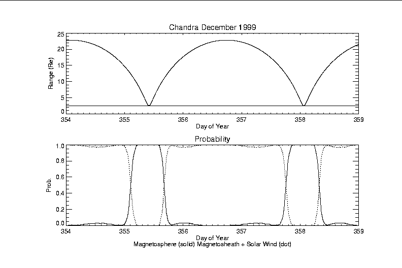
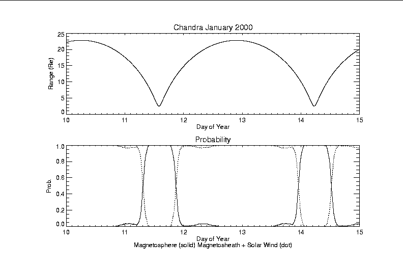
| Dec 1999 days 354-359 | Jan 2000 days 010-015 |
Data tables (gzip'd, try shift-click if your browser is prone to gunzip'ing) for 1999 November, 1999 December, and 2000 January are also available. The tables include time (YYYY MM DD HH MM SEC), decimal day-of-year, GSE X, Y, and Z spacecraft coordinates (in units of Re), the spacecraft range (in units of Re), and the probabilities the spacecraft is in each of the three regions, magnetosphere, magnetosheath, and solar wind, respectively.
Summaries of these probability tables for 1999 November, 1999 December, and 2000 January provide quick tabulations of the main features. Each of these files contain (a) a performance summary listing the observation and safing durations in days as functions of probability threshold, and (b) tables of entry and exit times (in day-of-year) with corresponding GSE X, Y, and Z coordinates and range (all in Re). Tables are included for each step in the probability threshold from 0.05 to 0.95 in increments of 0.05.
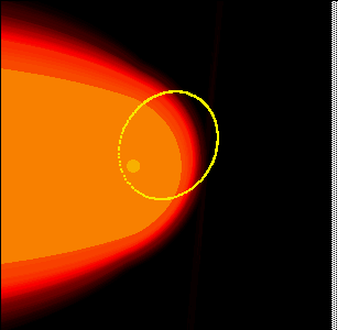
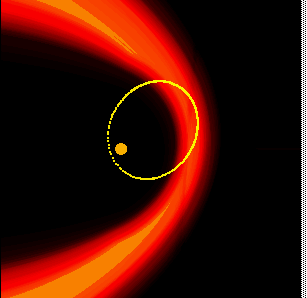
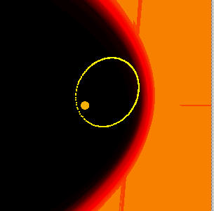
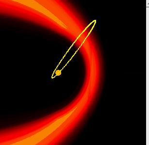
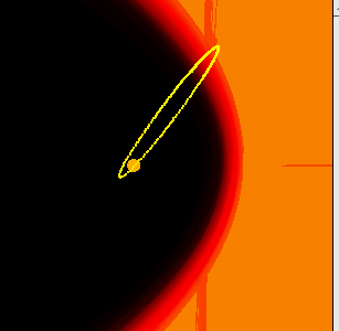
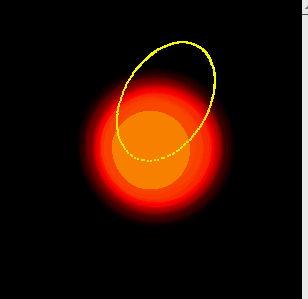
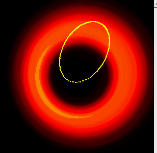
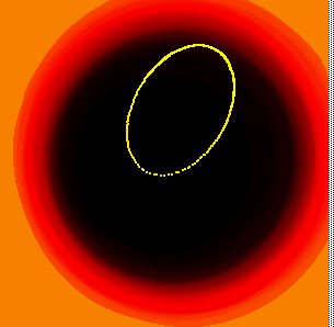
In addition to tables of region probabilities along the satellite's orbit, probability scenes are given below in the GSE coordinate system XY, XZ, and YZ planes (click on the thumbnail links to obtain the individual GIF file). Each scene represents a 50x50 Re spatial extent overlaid with Earth's location and a projection of a sample Chandra orbit. Probabilities for each region are color coded with black representing the lowest probability (0%) and light orange the highest probability (100%). The scenes provide a quick visualization of the orbit's intersection with the predicted magnetopause crossings and aid in simulation verification.
(NOTE: The apparent linear region of decreased probability in the solar wind plots is an artifact and should be ignored in these preliminary results.)
|
|
|
| Magnetosphere: XY GSE plane | Magnetosheath: XY GSE plane | Solar Wind: XY GSE plane |
|
|
|
| Magnetosphere: XZ GSE plane | Magnetosheath: XZ GSE plane | Solar Wind: XZ GSE plane |
|
|
|
| Magnetosphere: YZ GSE plane | Magnetosheath: YZ GSE plane | Solar Wind: YZ GSE plane |
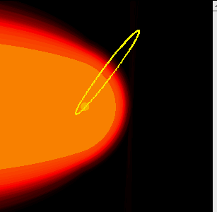
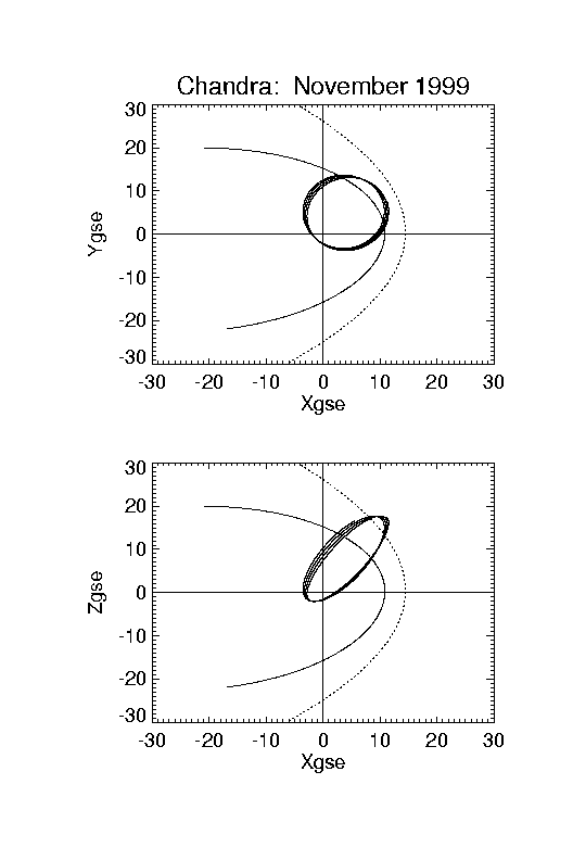
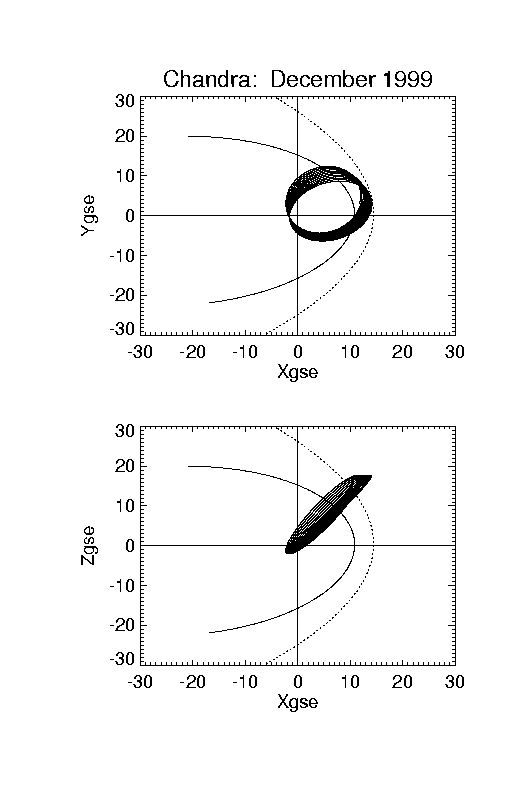
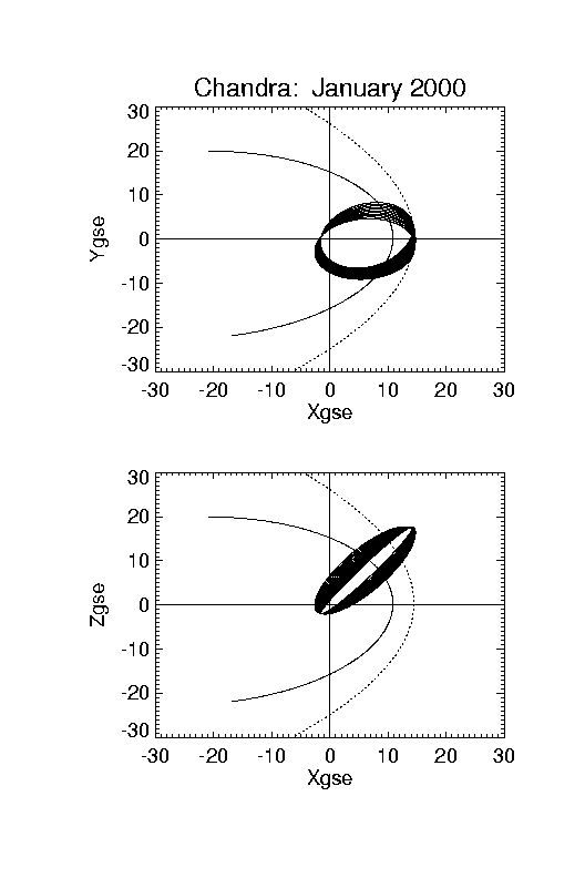
Orbits in the GSE coordinate system are given in the following. The magnetopause and bow shock positions in these figures are nominal values taken from the paper by Fairfield (1971) and are included here for reference. Note that during November Chandra was sampling the post-noon sector of the magnetosphere but by January it will be located in the daytime sector.
|
|
|
| November 1999 | December 1999 | January 2000 |
Examination of the orbit propagator for short- and long-term precision
in trajectory calculations and standardization with the current
"official" Chandra ephemerides.
Validation of the phenomenology models.
Enhancement of the solar wind database to include longer time series of IMP-8 data and/or data from the ACE satellite.
Comparison of probability results to EPHIN data for model verification and to determine if the EPHIN rates inside and outside the magnetosphere can be predicted with the tool.
Incorporate a proton model to treat particle flux variations inside the magnetosphere for use when Chandra spends significant time inside the magnetopause.
Return to our ACIS page, go to the Chandra Project Science Page or to X-ray Astronomy at MSFC
|
Editor: Dr. Douglas Swartz System Administrator: Mr. Bob Dean Privacy Policy and Important Notices Accessibility Statement |

|
|